Explaining Loss Functions - Part 1

Loss Functions

A loss function lies at the heart of most of the Machine Learning (ML) algorithms. For a newbie, the loss functions are a bit daunting. I struggled initially to come to terms with it. In most articles, the mathematics behind is explained but not the intuition. This is an attempt to make loss functions approachable. I really hope this helps a ML newbie.

Let’s understand loss: It is just the difference between the predicted value by the model and the actual value. The lesser the difference (loss), the better the model. That’s all there is to it. The model actually learns by reducing the loss and this is called training.

There are different ML tasks such as classification, regression etc., The way we measure the ‘difference’ varies for each task. That is why each task has its own loss function.

Let’s start with Cross Entropy and Mean Squared Error, used in classification and regression respectively.

Cross Entropy

Let’s consider a binary classification problem (2 classes, cat vs dog), the actual labels being 0 for cat and 1 for dog. Now the model is trained to predict a probability between 0 and 1. If the model produces a higher probability (let’s say 0.9) for dog and a lesser probability for cat (let’s say 0.1) the loss is lower.

On the other hand if the model produces 0.9 for cat, the loss should be higher. Of course, a perfect model will produce 0 for cat and 1 for dog. Any function that captures this characteristic can be considered as a loss function for classification.

Now a bit of mathematics! Cross entropy is calculated by the equation -

$$-<!--\; -\; -->(y\log <!--\; \; -->(p)+(1-<!--\; -\; -->y)\log <!--\; \; -->(1-<!--\; -\; -->p))$$

Here: p –> predicted probability
y –> actual label(s)

Here is the python implementation using numpy.

import numpy as np
def CalculateEntropyLoss(p, y):
    loss = -(y * np.log(p) + (1-y) * np.log(1-p) )
    return loss

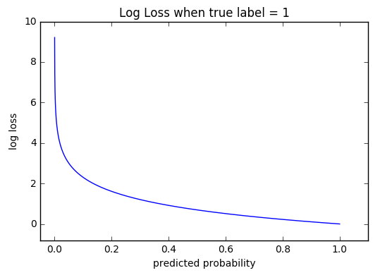
Now, Let’s unpack this equation with an example. For a dog, the actual label is 1. If the predicted probability is 0.1, the resultant loss from the above equation is 2.3. If the probability is 0.9, the loss is 0.1. You can see that this function fits our bill, the loss reduces as the predicted value is closer to actual value. You can try on your own. It works the other way as well.

You can learn more here

The example code is here

One more thing to note: Because of the log, the losses actually increase at log scale when the predictions move towards the wrong side. This can be seen in the plot below.

penalized more closer to 0 - from mlcheatsheet site

Mean Squared Error (MSE)

A regression task predicts a continuous variable. A squared error is a commonly used loss function in this task. As the name suggests, it is a mean of the squared error. The error is the difference between the actual value and the prediction, the error being squared to remove the -ve sign and then averaged for MSE.

Another reason for squaring the loss is that it produces a continuous convex function where Gradient Descent can be applied for learning. More on this in another article.

It is comparatively simpler to understand than Cross Entropy. Here is the python implementation.

import numpy as np
def CalculateRMSE(p, y):
  size = y.size
  loss = np.sum((p - y)**2) / size
  return loss

You might have noticed L2 norm or Euclidean norm mentioned in papers, it just means RMSE.

Mean Absolute Error (MAE)

It’s similar to MSE, instead of squaring the error, the absolute value of the error is considered. This is also called L1 or Manhattan Norm.

Another thing to note is that the RMSE is highly sensitive to outlier values as you would have guessed. This is because the square term. If the dataset has more outliers, prefer MAE. Otherwise, MSE works great!